Interactive apps for teaching
This
page contains a collection of interactive computer simulations or
calculations that I have found useful for teaching physics. They are
all written using Geogebra,
a freely available software package for learning and teaching
mathematics.
Each
app is available in two versions. The .html version will run
in a
browser window, without the installation of the Geogebra software.
All interactive features are available, but you cannot see or
modify the source code. On some computers certain apps refuse to run
for unknown reasons. The .ggb version is the original
Geogebra
file. To use it you must download the Geogebra software from the website. This
method is more reliable (though still not infallible) and gives you
full access to the underlying code.
If you try any of these, please send me an email with your reactions, comments, suggestions, or questions.
Math
 This
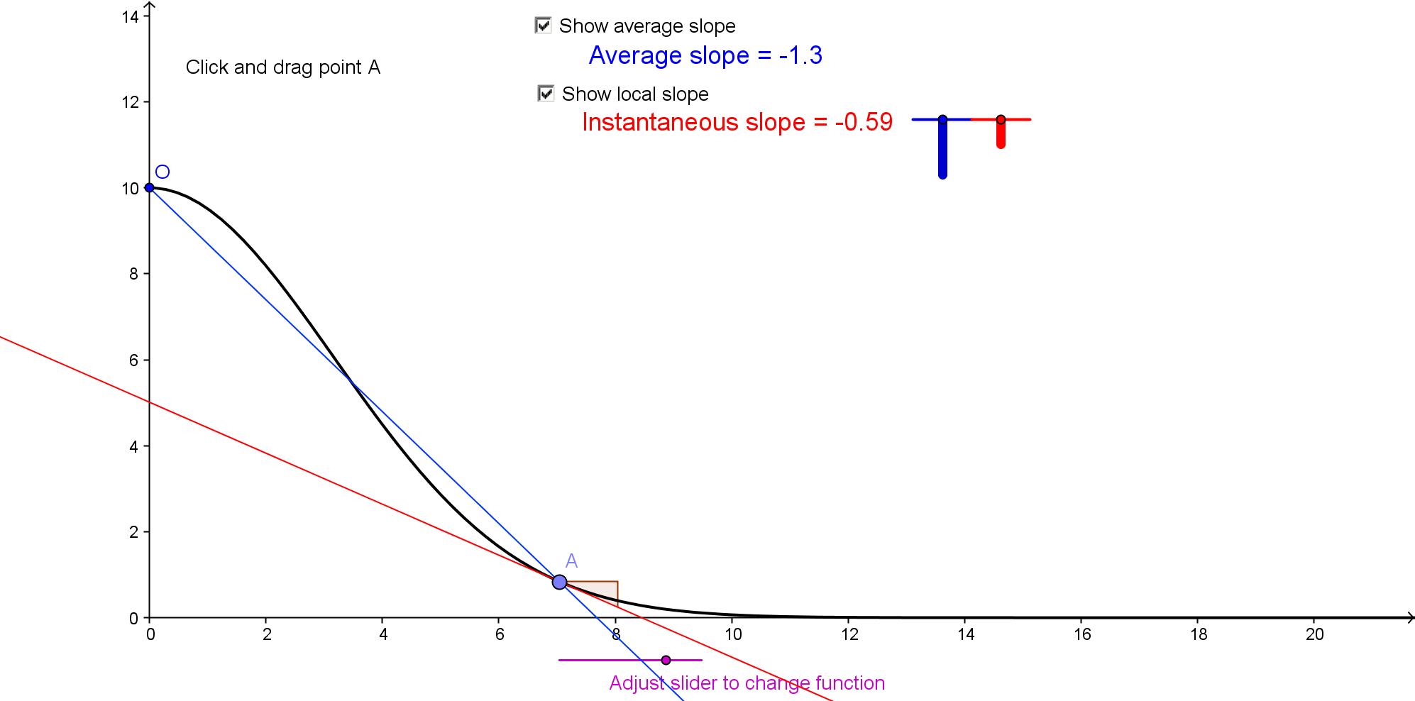
app is designed to help students explore and understand the ideas of
average and local slope (derivative) of a function.
This
app is designed to help students explore and understand the ideas of
average and local slope (derivative) of a function.
html version
ggb version
Top
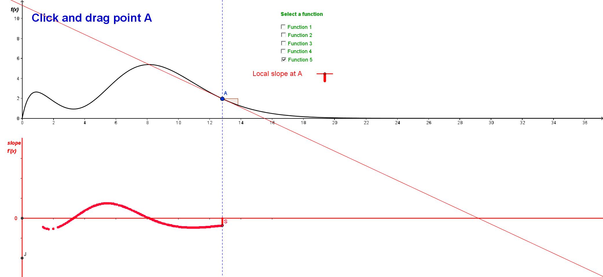 This app is
designed to help students explore and understand the relationship
between a function and its derivative.
This app is
designed to help students explore and understand the relationship
between a function and its derivative.
html version
ggb version
Top
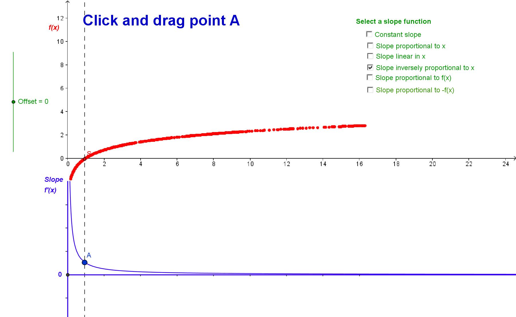 This app is
designed to help students explore and understand the relationship
between a function and its integral.
This app is
designed to help students explore and understand the relationship
between a function and its integral.
html version
ggb version
Top
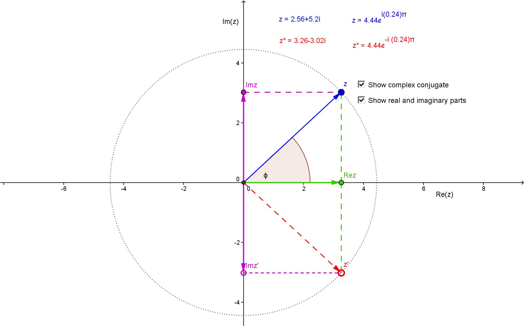 This app explores
the various representations of a complex number, and its relationship
to its complex conjugate.
This app explores
the various representations of a complex number, and its relationship
to its complex conjugate.
html version
ggb version
Top
Waves and Quantum Mechanics
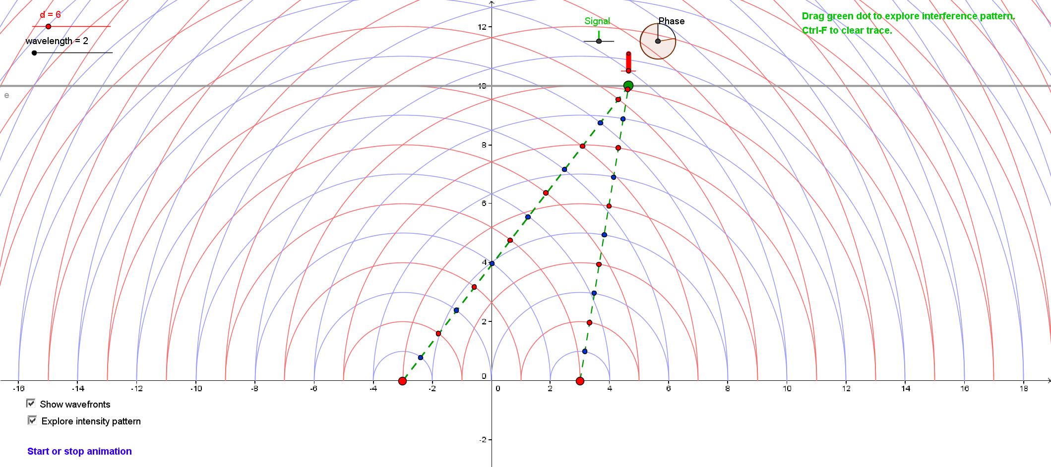 This
app simulates interference between the waves from two in-phase sources.
It can display both the wavefronts and the interaction of the waves at
a particular point on the screen, and allows tracking of the
interference pattern.
This
app simulates interference between the waves from two in-phase sources.
It can display both the wavefronts and the interaction of the waves at
a particular point on the screen, and allows tracking of the
interference pattern.
html version
ggb version
Top
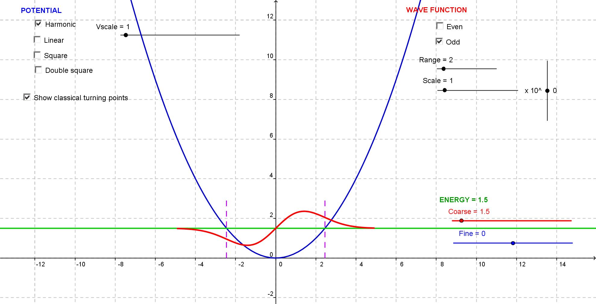 This
app uses the "wag the dog" method (see D.J. Griffiths, Introduction to Quantum Mechanics,
ch. 2) to find approximate energy eigenstates and eigenvalues for
various one-dimensional potentials.
This
app uses the "wag the dog" method (see D.J. Griffiths, Introduction to Quantum Mechanics,
ch. 2) to find approximate energy eigenstates and eigenvalues for
various one-dimensional potentials.
html version
ggb version
Top
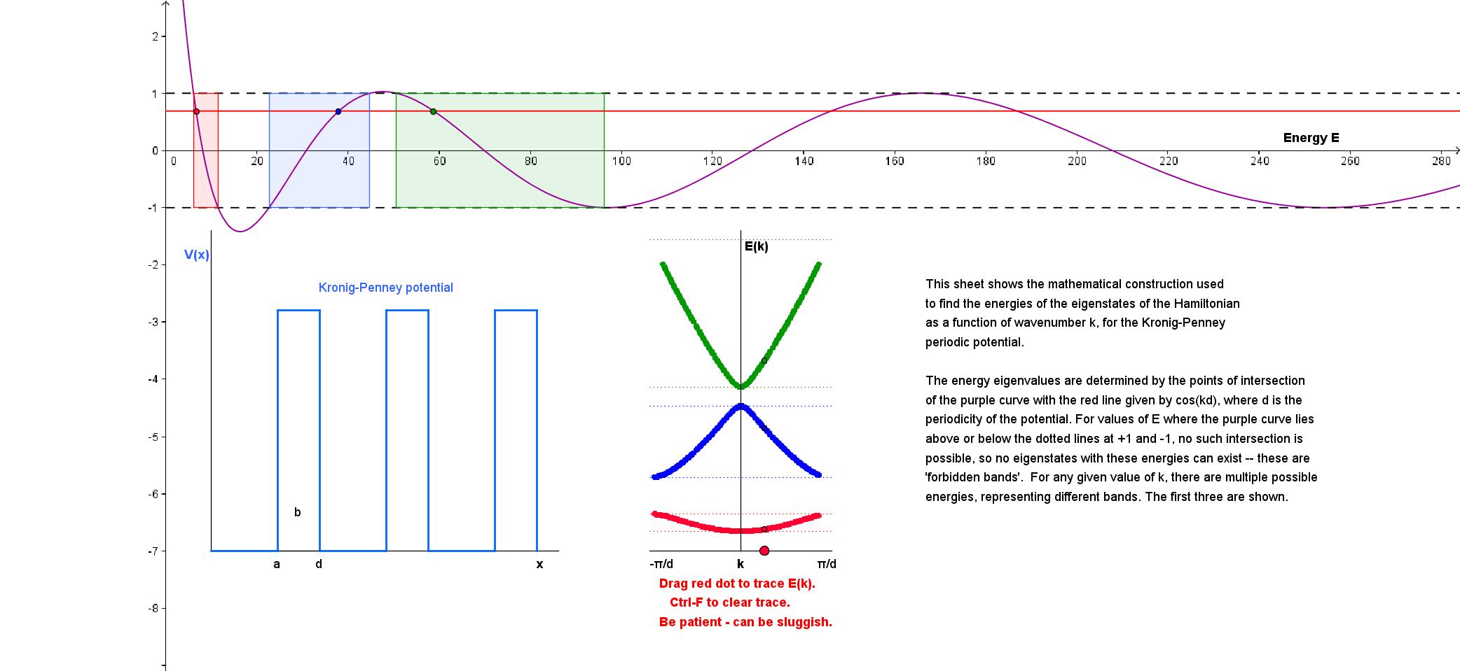 The
analysis of the Kronig-Penney model of a one-dimensional solid leads to
a rather opaque equation that implicitly gives the dispersion relation
E(k), but can only be solved numerically (see R.L. Liboff, Introductory Quantum Mechanics,
Ch. 8). This app provides some clarification of at least the
mathematical problem, and allows you to trace out the E(k) curve for
the three lowest bands.
The
analysis of the Kronig-Penney model of a one-dimensional solid leads to
a rather opaque equation that implicitly gives the dispersion relation
E(k), but can only be solved numerically (see R.L. Liboff, Introductory Quantum Mechanics,
Ch. 8). This app provides some clarification of at least the
mathematical problem, and allows you to trace out the E(k) curve for
the three lowest bands.
html version
ggb version
Top
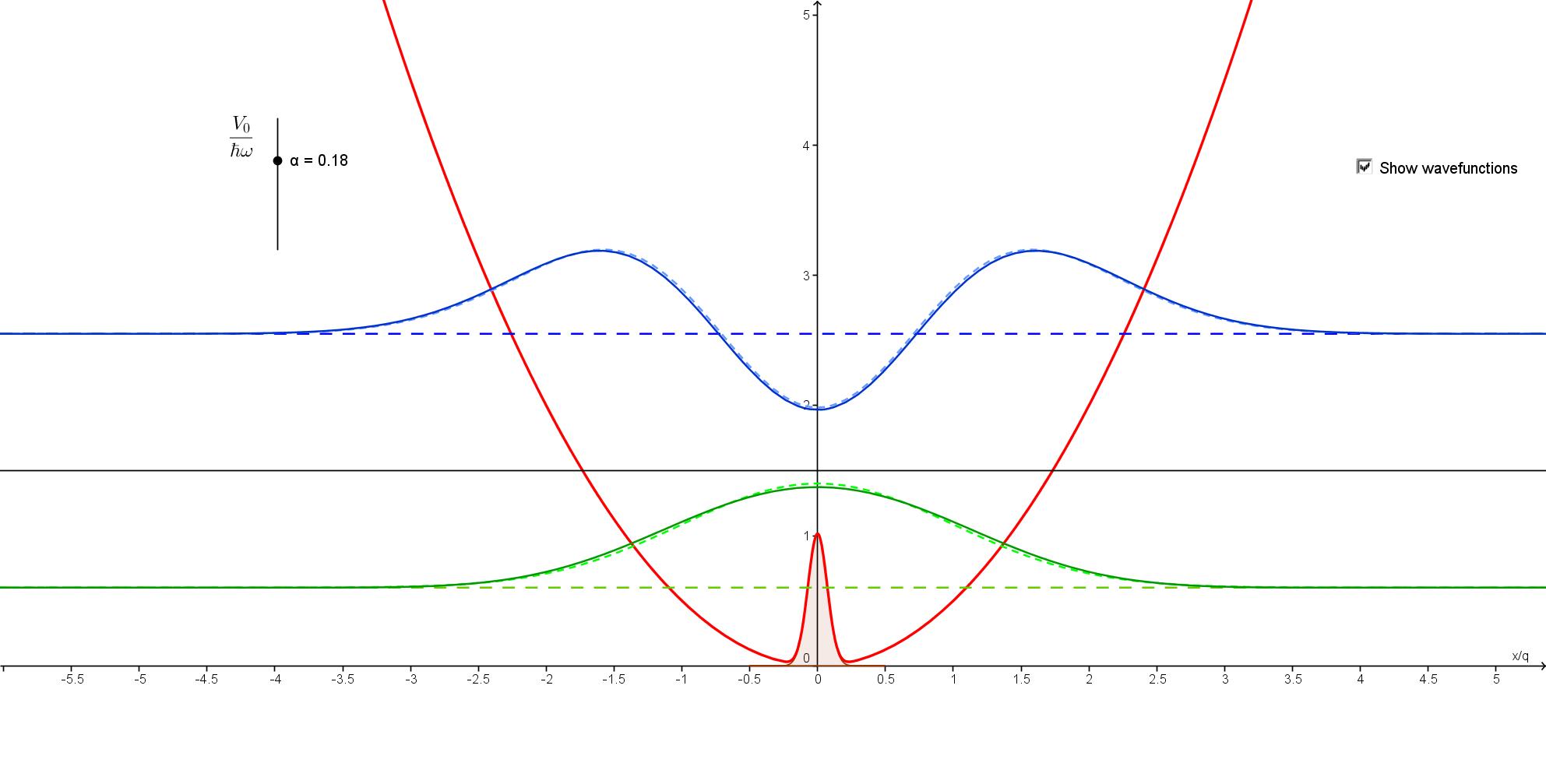 Shows
the effect of a simple perturbation on the energies and wavefunctions
of the two lowest states of a one-dimensional harmonic oscillator.
Shows
the effect of a simple perturbation on the energies and wavefunctions
of the two lowest states of a one-dimensional harmonic oscillator.
html version
ggb
version
Top
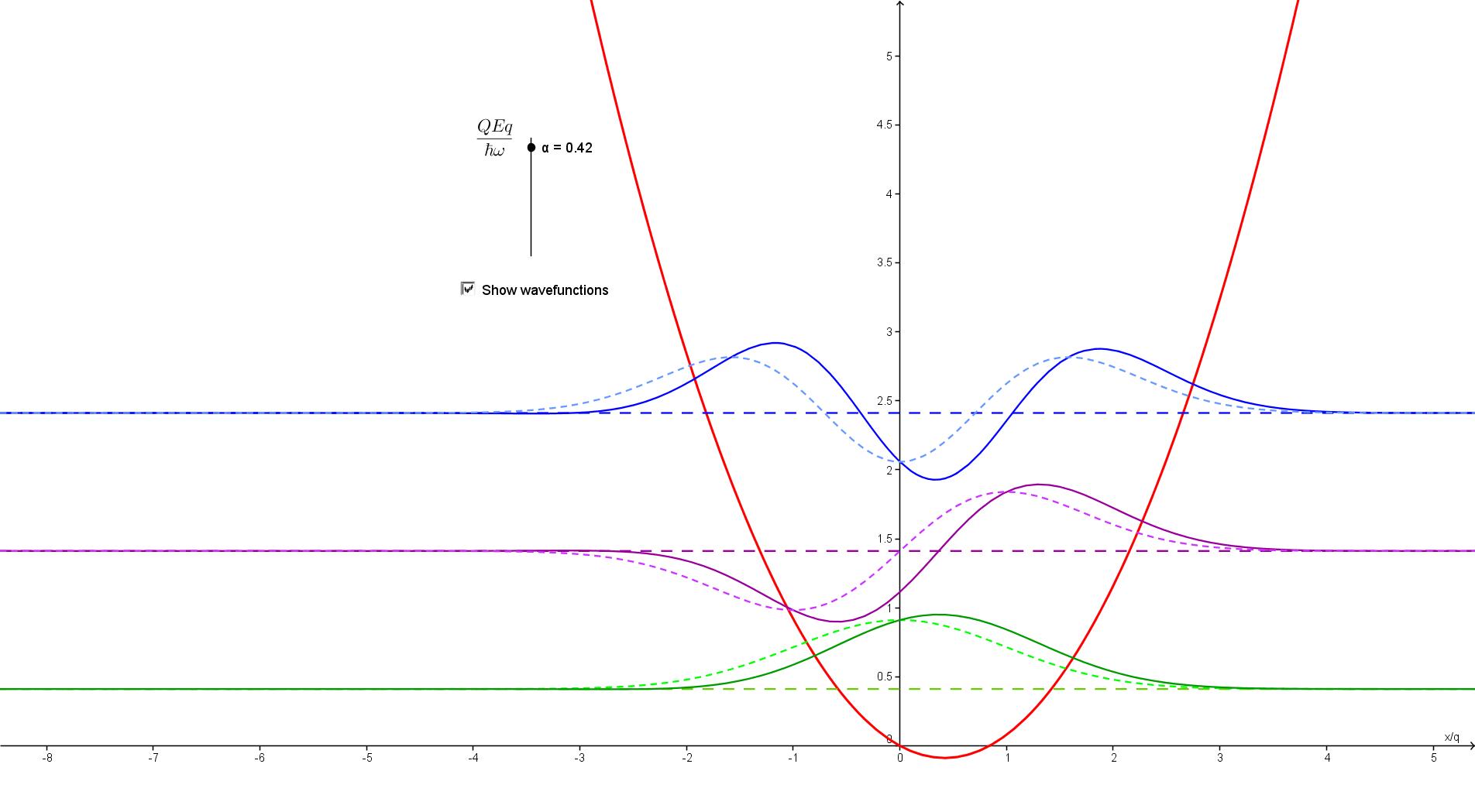 Shows
the effect of a linear perturbation on the energies and wavefunctions
of the three lowest states of a one-dimensional harmonic oscillator,
calculated in second-order perturbation theory.
Shows
the effect of a linear perturbation on the energies and wavefunctions
of the three lowest states of a one-dimensional harmonic oscillator,
calculated in second-order perturbation theory.
html version
ggb
version
Top
TopTop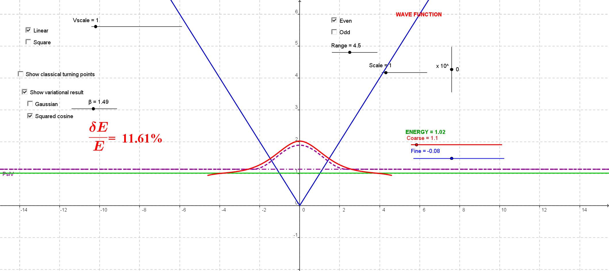 This
is a modified version of the "wag the dog" app above, intended to
illustrate the variational approximation method. You can use the "wag
the dog" method to find the energy and wavefunction for the first or
second eigenstate of a linear or square potential, and then find the
best variational approximation to the state using a trial wavefunction
based either on a Gaussian or a cosine-squared function.
This
is a modified version of the "wag the dog" app above, intended to
illustrate the variational approximation method. You can use the "wag
the dog" method to find the energy and wavefunction for the first or
second eigenstate of a linear or square potential, and then find the
best variational approximation to the state using a trial wavefunction
based either on a Gaussian or a cosine-squared function.
html version
ggb version
Top
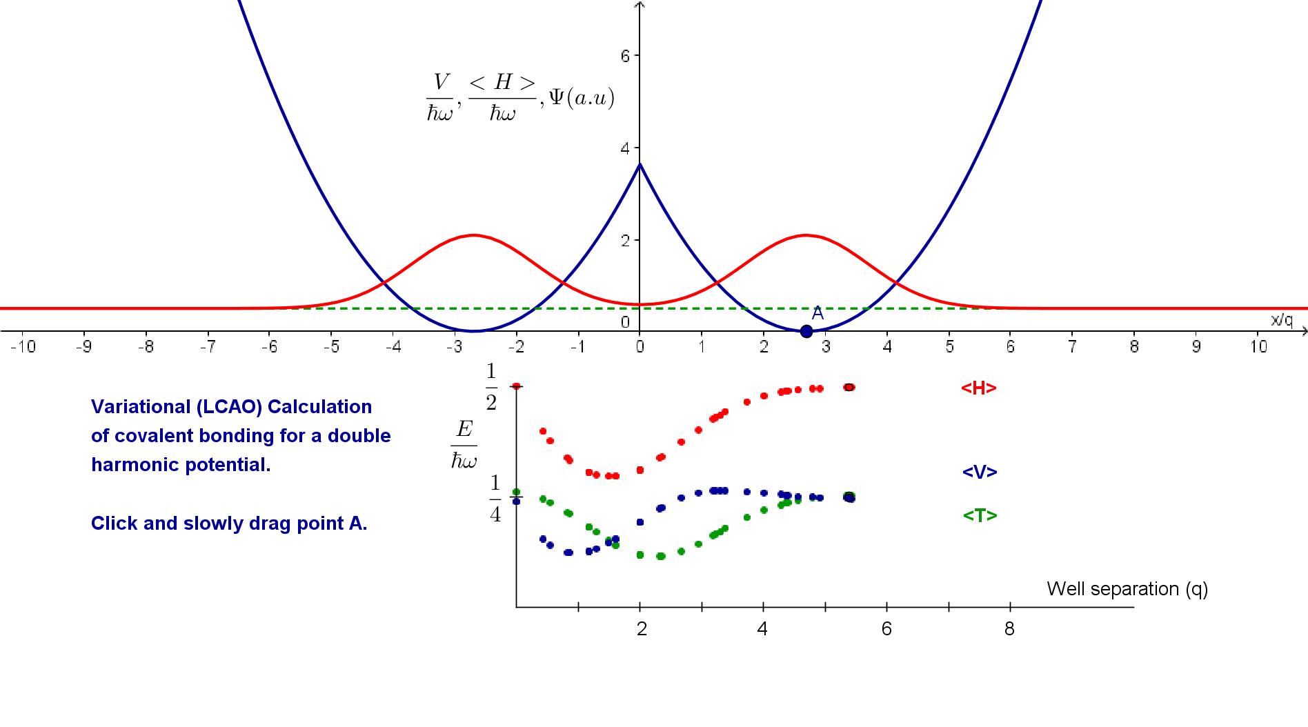 This
app illustrates the LCAO (linear combination of atomic orbitals)
approximation method in a simple 1-D case. The potential is double
harmonic well, and the wavefunction is the sum of two Gaussians
centered at the well minima. The only variable is the well separation.
As you drag the point at the bottom of one well, the expectation values
of the kinetic energy <T>, potential energy
<V> and total
energy <H> are graphed; the presence of a minimum shows
that
there is a bound state. Because the program is doing a lot of
integrating, the response time is slow, and you have to be patient.
This
app illustrates the LCAO (linear combination of atomic orbitals)
approximation method in a simple 1-D case. The potential is double
harmonic well, and the wavefunction is the sum of two Gaussians
centered at the well minima. The only variable is the well separation.
As you drag the point at the bottom of one well, the expectation values
of the kinetic energy <T>, potential energy
<V> and total
energy <H> are graphed; the presence of a minimum shows
that
there is a bound state. Because the program is doing a lot of
integrating, the response time is slow, and you have to be patient.
html version
ggb version
Top